Definitions
EOQ generally minimizes the total inventory cost. However, EOQ may not be optimal when discounts are factored into the calculation.
The optimal order quantity when discounts are involved is either:
- EOQ; or
- Any one of the minimum order quantities above EOQ that qualify for additional discount.
The optimum quantity is determined by comparing the total inventory cost of the different order quantities listed above.
For example, if the EOQ is 1000 units and discounts of 2%, 5% and 8% are offered at 500 units, 1000 units and 2000 units, the order quantity that shall lead to the lowest total inventory cost will either be the EOQ (i.e. 1000 units) or 2000 units. In order to determine the optimum quantity, we need to compare the total inventory cost of order quantities of 1000 units and 2000 units. We can ignore the total inventory cost of 500 units as it is below the EOQ level.
Example
- 2% discount on orders above 200 units
- 4% discount on orders above 500 units
- 6% discount on orders above 600 units
- Annual demand is 5000 units
- Ordering cost is $100 per order
- Annual holding cost is comprised of the following:
- 5% insurance premium for the average inventory held during the year calculated using the net purchase price
- Warehousing cost of $6 per unit
- Purchase price is $200 per unit before discount
Solution
We need to compare the total inventory cost of the order quantities at the various discount levels with that of the economic order quantity.
Since the holding cost is partially determined on the basis of purchase price, we need to re-calculate the EOQ by applying a discount. As the EOQ seems likely to fall within the 200 to 400 units range, we should use 2% discount in our calculation.
EOQ = √(2 x 100 (Order Cost) x 5000 (Annual Demand)) / (0.05x( 200×0.98) + 6 (Holding Cost))
≈ 252 units
| Order Quantity | 252 units | 500 units | 1,000 units |
|---|---|---|---|
|
Number of orders (Annual demand ÷ Order Quantity) |
5,000 ÷ 252 = 19.84 |
5000 ÷ 500 = 10 |
5,000 ÷ 1,000 = 5 |
|
Ordering Cost (number of orders × $100) |
19.84 x 100 = $1,984 |
10 x 100 = $1,000 |
5 x 100 = $500 |
|
Warehousing Cost ($6 × Average number of units) |
6 × 252/2 = $756 |
6 × 500/2 = $1,500 |
6 × 1000/2 = $3,000 |
|
Insurance Cost (5% × Purchase Price × Average Inventory) |
0.05 × (200×0.98) × (252/2) = $1,235 |
0.05 × (200×0.96) × (500/2) = $2,400 |
$0.05 × (200×0.94) × (1000/2) = $4,700 |
|
Cost of Purchase (Purchase Price × Annual Demand × (100 - discount%) |
200 × 5000 × (1.0-0.02) = $980,000 |
200 × 5000 × (1.0-0.04) = $960,000 |
200 × 5000 × (1.0-0.06) = $940,000 |
|
Total Inventory Cost |
$983,975 |
$964,900 |
$948,200 |
Based on the above analysis, the optimum order quantity is 1000 units.
Note:
You may be wondering whether increasing the order size from 1000 units will result in more savings. The short answer is no. The behavior of inventory cost can be illustrated in the following graph.
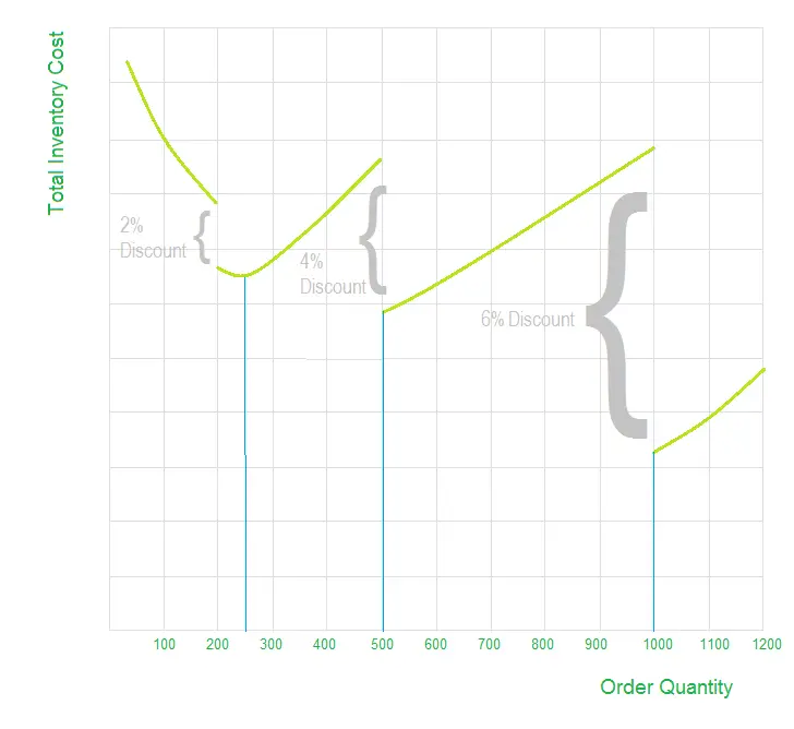
There is a pattern of stepped decrease in total inventory cost after every discount slab is reached followed by gradual increase in the cost. As noted earlier, whenever discounts are offered, the optimum order quantity will be either the EOQ or one of the minimum discount quantities above the EOQ level (i.e. 252 units, 500 units or 1000 units in the example above). Any quantity above or below these quantities will result in an increase in the total inventory cost and should therefore be ignored.