Definitions
Economic Order Quantity (EOQ) is the order quantity that minimizes total inventory costs.
Order Quantity is the number of units added to inventory each time an order is placed.
Total Inventory Costs is the sum of inventory acquisition cost, ordering cost, and holding cost.
Ordering Cost is the cost incurred in ordering inventory from suppliers excluding the cost of purchase such as delivery costs and order processing costs.
Holding Cost, also known as carrying cost, is the total cost of holding inventory such as warehousing cost and obsolescence cost.
Explanation
Total inventory cost is comprised of the following main costs:
- Cost of purchase
- Order Costs
- Holding Costs
If we change the order quantity, it can affect the different types of inventory costs in different ways.
Larger order size results in lower order costs because fewer orders need to be placed to cover the annual demand. This however results in higher holding costs because of the increase in inventory levels.
Conversely, smaller order size results in lower holding costs because of the decline in average inventory level. However, as lower quantity of inventory is ordered each time, the number of orders needed to increase in order to fulfill the annual demand which leads to higher ordering costs. Reducing the order size may also affect the cost of purchase due to the loss of trade discounts that are based on the order quantity.
So the question arises how we can find the optimal order quantity that minimizes the total inventory costs.
EOQ model offers a method of finding the optimal order quantity that minimizes inventory costs by finding a balance between the opposing inventory costs.
Formula
Economic Order Quantity = √ ( 2 × Co × D / Ch )
Where:
- Co is the cost of placing one order
- D is the annual demand
- Ch is the annual cost of holding one unit of inventory
How is the EOQ formula derived?
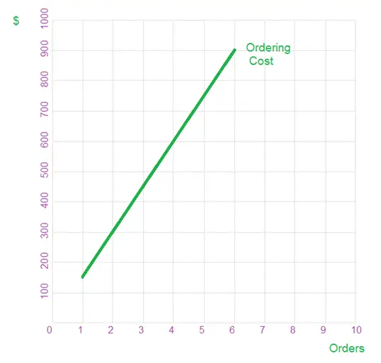
Ordering Costs increase linearly with an increase in number of orders, e.g. if one order costs $150 to process, 2 orders will cost $300 and so on. If we plot this information for a number of orders on the graph, it will appear as follows.
| Orders | Orders Cost |
|---|---|
|
1 |
$150 |
|
2 |
$300 |
|
3 |
$450 |
|
4 |
$600 |
|
5 |
$750 |
|
6 |
$900 |
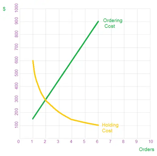
Holding costs on the other hand decrease with an increase in number of orders because doing so reduces the average units of inventory ordered and therefore held.
To illustrate, let’s assume that annual demand is 12000 units and it costs 10 cents for holding one unit of inventory for one year. If only one order is placed at the start of the year, the order quantity needs to be 12000 units to meet the demand for the whole year. The inventory units on the first day of the year will be 12000 units and it will gradually reduce to zero units on the last day of the year. The average inventory will be in between the two extremes, i.e. 6000 units ( (12000 + 0) ÷ 2). The annual holding cost will therefore be $600 (6000 x $0.1) if only one order is placed.
Now if the number of orders is increased to two, the average inventory will reduce to half along with the annual holding cost.
If we plot this information against 6 orders on the graph, it will appear like this:
| Orders | Order Quantity | Average Inventory | Holding Costs |
|---|---|---|---|
|
|
(12000 ÷ Orders) |
(Order Quantity ÷ 2) |
($0.1 x Average Inventory) |
|
1 |
12,000 |
6,000 |
$600 |
|
2 |
6,000 |
3,000 |
$300 |
|
3 |
4,000 |
2,000 |
$200 |
|
4 |
3,000 |
1,500 |
$150 |
|
5 |
2,400 |
1,200 |
$120 |
|
6 |
2,000 |
1,000 |
$100 |
If we combine both costs we can calculate the total cost for each order level.
| Orders | Order Cost | Holding Costs | Total Costs |
|---|---|---|---|
|
1 |
$150 |
$600 |
$750 |
|
2 |
$300 |
$300 |
$600 |
|
3 |
$450 |
$200 |
$650 |
|
4 |
$600 |
$150 |
$750 |
|
5 |
$750 |
$120 |
$870 |
|
6 |
$900 |
$100 |
$1,000 |
The lowest total cost occurs where order costs and holding costs are the same. This is illustrated in the following graph where the lowest point of the total cost curve matches the point where order cost and holding costs connect.
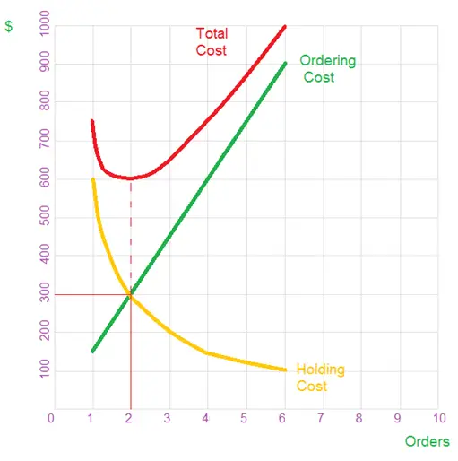
We can deduce from the above graph that the total inventory cost will be minimum where Ordering Costs = Holding Costs.
If we assume that the variables that determine the ordering cost and holding cost other than the order quantity are constant (i.e. annual demand, holding cost of one unit, cost of 1 order), we can substitute these values in the equation Ordering Costs = Holding Costs and find the missing quantity (EOQ) using simple algebra as follows.
Holding Cost = Order Cost
Average Quantity x Holding Cost per Unit = Number of Orders x Order Cost
(Quantity / 2) x Holding Cost per Unit = (Demand / Quantity) x Order Cost
Quantity x Quantity x Holding Cost per Unit = 2 x Demand x Order Cost
Quantity2 = (2 x Demand x Order Cost) / Holding Cost per Unit
Quantity = √ ( 2 × Co × D / Ch )
Relevant Costs
When calculating EOQ, it is important to include only those ordering and holding costs that are relevant. Any costs that are not incremental should be ignored while calculating EOQ. Following examples illustrate the application of relevant costing in the calculation of EOQ.
| Order Costs | Relevance to EOQ calculation |
|---|---|
|
Salary paid to clerk who processes orders. |
If increase in number of orders would not result in overtime or hiring an additional clerk, the cost will not be relevant to EOQ. |
|
Supplier charges $5 delivery cost for each unit of inventory supplied. |
The total delivery expense will be the same irrespective of the number of order deliveries so it should be ignored in EOQ calculation. |
|
Supplier charges $500 fixed delivery charge for each delivery. |
Delivery expense will increase with an increase in number of orders so it should be included in EOQ calculation. |
|
Auto dealer transports cars from the car factory to its showroom using its own trucks. Insurance premium is paid to cover for any accidents during the transportation. $100 premium is paid for each vehicle that is transported. |
The annual insurance cost is fixed irrespective of how many cars are transported in one go and should therefore be ignored. |
| Holding Costs | Relevance to EOQ calculation |
|---|---|
|
Company earns a return of 15% on its projects. One unit of inventory costs $100. |
The opportunity cost of holding one more unit of inventory for one year is $15(15%x$100) which should be included in EOQ calculation because more the number of units of inventory that are held, higher the opportunity cost of capital tied in inventory purchase. |
|
Company pays lease rentals of $20,000 for its warehouse. |
Warehouse rent is fixed and hence irrelevant to EOQ calculation as the cost does not vary to changes in the number of units of inventory held. |
|
Insurance premium of $10 per day is paid for each unit of inventory stored in the warehouse to cover the risk of fire and theft. |
The insurance cost rises with an increase in number of units held and is therefore relevant to EOQ. |
|
0.2% of the average number of inventory units stored in the warehouse get damaged or stolen. |
The cost of damage and shrinkage (theft) of inventory increases as more units of inventory are held at the warehouse. The cost should therefore be factored into EOQ calculation. |
Example
Jason owns a fish shop where he sells an exotic variety of tuna fish which he imports from Japan.
Jason refrigerates the fish in a cold storage facility near his shop that charges him a fixed annual fee of $1000 and variable charge of $5 per day for each fish container that is stored.
Every morning, Jason brings fish from the cold storage to his shop for sale. Jason estimates that he incurs $10,000 electricity cost each year on refrigerating the fish inside his own shop.
Jason incurs the following ordering costs:
- Delivery charges of $10,000 per delivery
- Import duties of $300 per carton
- Custom fees of $200 per order
- Import license fee of $150 per annum
Jason currently imports fish by placing one order of 20 cartons every month. Each carton costs $2,000.
Jason is wondering if he can save inventory costs by adopting EOQ model.
a) Calculate the current annual total inventory costs
b) Calculate the economic order quantity
c) Calculate the annual total inventory costs if EOQ is used
Solution
a) Current Inventory Cost
| Costs | Working | $ |
|---|---|---|
|
Purchase Cost |
Annual demand = 20 x 12 = 240 cartons
Purchase cost = 240 x $2000 = $480,000 |
480,000 |
|
Order Cost |
|
|
|
Delivery Cost |
Number of deliveries = 12 |
120,000 |
|
Import Cost |
Import fee = $300 x 240 cartons = $72,000 |
72,000 |
|
Custom Cost |
Custom fee = $200 x 12 orders = $2400 |
2,400 |
|
Holding Cost |
|
|
|
Cold storage |
Maximum number of cartons stored = 20 |
19,250 |
|
Electricity |
|
10,000 |
|
Total Inventory Cost (Current) |
703,650 |
|
b) Economic Order Quantity
EOQ = √ ( 2 x 10,200 (W1) x 240 (W2) ) / ( 1,825 (W3) )
≈ 52 cartons
Order Cost (W1)
Delivery Cost $10,000
Import fees –
Custom fees $200
Cost of 1 order $10,200
Note:
Import fees can be ignored in EOQ calculation as they remain the same irrespective of the number of orders.
Annual Demand (W2) = 240 cartons
Holding Cost (W3)
Cold Storage: Variable (365 x $5) $1,825
Cold Storage: Fixed –
Electricity –
Cost of holding 1 carton for 1 year = $1,825
c) Inventory Cost using EOQ
| Costs | Working | $ |
|---|---|---|
|
Purchase Cost |
As before |
480,000 |
|
Order Cost |
|
|
|
Delivery Cost |
Annual Demand = 240 cartons |
50,000 |
|
Import Cost |
As before |
72,000 |
|
Custom Cost |
Custom fee = $200 x 5 orders = $1000 |
1,000 |
|
Holding Cost |
|
|
|
Cold storage |
Maximum number of cartons stored = 52 |
19,250 |
|
Electricity (as before) |
|
10,000 |
|
Total Inventory Cost (using EOQ) |
661,450 |
|
Using EOQ Model will save Jason $42,200 (703,650 – 661,450) annually.
Tip
Annual holding cost per unit is sometimes expressed as a percentage of the inventory purchase price.
Assumptions
- EOQ model assumes a constant demand.
- EOQ calculation assumes that ordering costs and holding costs will remain constant.
Limitations
- Since no fluctuation in demand is considered in the EOQ calculation, business losses due to potential shortage of inventory are ignored.
- EOQ model does not take into account the seasonal fluctuations in the cost of inventory. In seasonal industries, it would make sense to buy inventory in bulk when it is readily available at a lower price. Inventory may be harder to procure in off season and would usually cost more as well.
- EOQ model does not take into account purchase discounts that could be obtained by buying inventory in bulk. We can however work around this problem as is illustrated in this next lesson.