Bob, a farmer, is wondering which crops he should plant in the upcoming season.
He can grow wheat and barley on his 4000 acres of farmland.
Bob uses only organic fertilizers on his farm. He estimates that a maximum of 10 Metric Tons of organic fertilizers could be procured for the upcoming season.
Bob is confused regarding which crop (or combination of crops) to grow in order to maximize his income because although wheat yields a relatively higher contribution, growing barley requires relatively less land and fertilizers compared to wheat.
Comparison of wheat and barley is as follows:
| Wheat (1 Metric Ton) | Barley (1 Metric Ton) | |
|---|---|---|
|
Contribution |
$200 |
$100 |
|
Land requirement |
1 acre |
0.8 acre |
|
Fertilizer requirement |
0.004 MT |
0.001 MT |
Find the optimum production plan that will maximize Bob’s income.
Step 1: Define Constraints
Variables used for constraints:
W = Quantity of wheat (in metric tons) to be grown
B = Quantity of barley (in metric tons) to be grown
- Land constraint 1W + 0.8B ≤ 4000
Explanation
Only such quantities of wheat and barley can be grown that their combined coverage of land does not exceed 4000 acres.
- Fertilizer constraint 0.004W + 0.001B ≤ 10
Explanation
Only such quantities of wheat and barley can be grown that their combined usage of fertilizers does not exceed 10 MT.
- Non-Negativity constraint W ≥ 0 and B ≥ 0
Explanation
Only positive quantities of wheat and barley can be grown.
Step 2: Define the Objective Function
Objective function: 200W + 100B = 1,000,000
Explanation
Since Bob’s objective is to maximize his income, we have used the contribution per unit of wheat and barley in the objective function.
1000000 is just a random number that we have used to obtain the slope of the objective function. Any other number could also be used as the gradient will remain the same.
Step 3: Plot the constraints on a graph paper
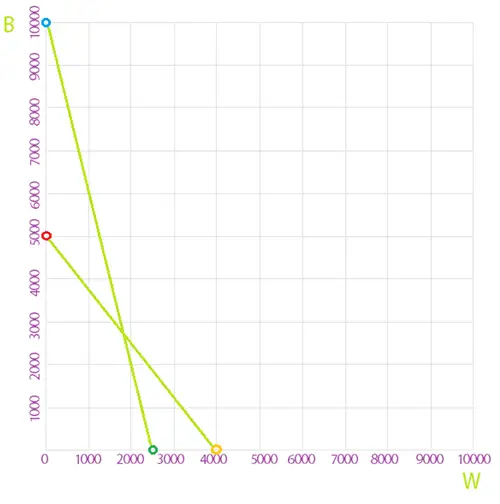
Working:
| Constraints | Wheat | Barley | Point 1 | Point 2 |
|---|---|---|---|---|
|
1W + 0.8B ≤ 4000 |
0 |
1(0)+0.8B =4000 |
(0, 5000) |
|
|
1W + 0.8(0) = 4000 |
0 |
|
(4000, 0) |
|
|
0.004W + 0.001B ≤ 10 |
0 |
0.004(0)+0.001B = 10 |
(0, 10,000) |
|
|
0.004W + 0.001(0) = 10 |
0 |
|
(2500, 0) |
Step 4: Highlight the feasible region on the graph
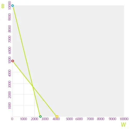
Feasible region is the white area on the graph.
Step 5: Plot the objective function on the graph
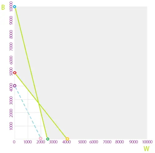
Working:
| Objective Function | W | B | Point 1 | Point 2 |
|---|---|---|---|---|
|
200W + 100B = 400000 |
0 |
0 + 100B =400000 |
(0, 4000) |
|
|
200W + 0 = 400000 |
0 |
|
(0, 2000) |
Step 6: Find the optimum point
![]() Optimum point always lies on one of the corner points of the feasible region.
Optimum point always lies on one of the corner points of the feasible region.
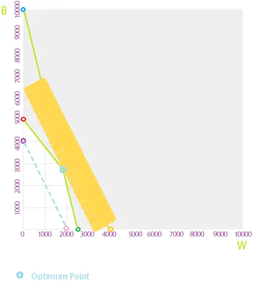
Step 7: Find the coordinates of the optimum point
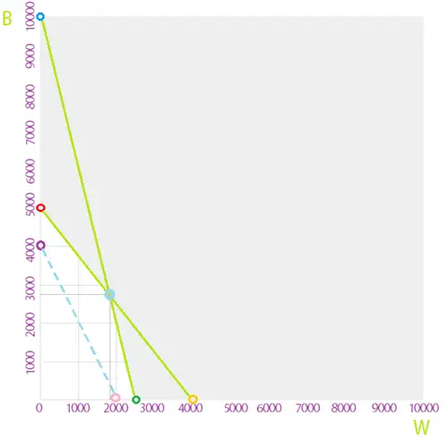
Co-ordinates of the optimum point are approximately 1850 W and 2750 B (1850, 2750).