Introduction
Graphical method of linear programming is used to solve problems by finding the highest or lowest point of intersection between the objective function line and the feasible region on a graph.
This process can be broken down into 7 simple steps explained below.
Step 1: Define Constraints
All constraints relevant to a linear programming problem need to be defined in the form of inequalities.
What are inequalities?
Inequalities are mathematical expressions similar to equations except for 1 difference. Unlike equations which state what is equal to something (e.g. x = y) , inequalities express what is greater or lesser than something (e.g. x > y).
Inequalities are stated using the following symbols:
> Greater than
≥ Greater or equal to
< Lesser than
≤ Lesser or equal to
Step 2: Define the Objective Function
The objective of solving a problem is expressed in the form of a mathematical equation.
For example, if the objective is to maximize contribution from the sale of Products A and B having contribution per unit of $10 and $5 respectively, the objective function shall be:
10A + 5B = Maximum Contribution
What this means is that the objective of solving the problem is to maximize the total contribution of the business by selling the optimum mix of products A and B.
The problem with the above equation is that we cannot simply plot it on a graph (as required in step 5). To work around this problem, we define a random number in place of ‘Maximum Contribution’. Since we only require the slope (gradient) of the objective function, we can plot the Objective Function on a graph using any random value in place of maximum contribution.
Using the earlier example, the objective function could be re-written as:
10A + 5B = 100
Note that the 100 above is just a random number. Any other value could also be used instead.
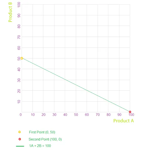
Step 3: Plot the constraints on a graph paper
Constraint inequalities, as defined in Step 1, should be plotted on a graph.
You may plot the constraints in the same manner as you would plot an equation.
Example
Constraint : 1A + 2B ≤ 100
For the purpose of plotting the above constraint on a graph, you may convert the inequality into an equation:
1A + 2B = 100
Now you need the co-ordinates of any 2 points from the above equation.
How do we find co-ordinates of a point from an equation?
In order to find the co-ordinates, simply insert a random value for either A or B. Solving the equation after inserting the random values could then be used to find the value of the other coordinate.
For example, we can find the value of B when A = 0 by inserting zero in place of A and solving the equation as follows:
1(0) + 2B = 100
0 + 2B = 100
2B = 100
B = 50
So the coordinates of the first point are A = 0 and B = 50 which can be written as
(0, 50).
Similarly, inserting zero as the value of B can give us the value of A for the second point as follows:
1A + 2(0) = 100
1A + 0 = 100
1A = 100
A = 100
Therefore, the coordinates of the second point are A = 100 and B = 0 or (100, 0).
Once you have determined the coordinates of any 2 points from the equation, you simply mark them on the graph and draw a straight line across them as shown below.
Step 4: Highlight the feasible region on the graph
Once you have plotted the constraint inequalities on the graph, you need to shade the area of the graph which is outside the constraint limits, i.e. which is not feasible.
For example, the constraint 1A + 2B ≤ 100 will be shaded as follows:
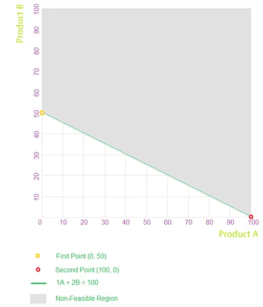
The area on graph which lies on or below the constraint limit line is feasible and therefore left un-shaded. Once all constraint limit lines have been similarly shaded, the non-shaded portion of the graph will represent the feasible region.
It can be confusing at times knowing which side of a constraint line to shade. In such cases, it is useful to consider whether a specific combination (e.g. 0 units of A, 0 units of B) above or below the line is possible or not considering that constraint only. If the combination is feasible, you must shade the opposite side of the line and vice versa.
Step 5: Plot the objective function on the graph
Objective Function line may be drawn on the graph in the same way as the constraint lines except that you may choose to differentiate it from constraint lines, e.g. by drawing a dotted line instead of the usual line.
Objective function line of 10A + 5B = 100 will be drawn as follows:
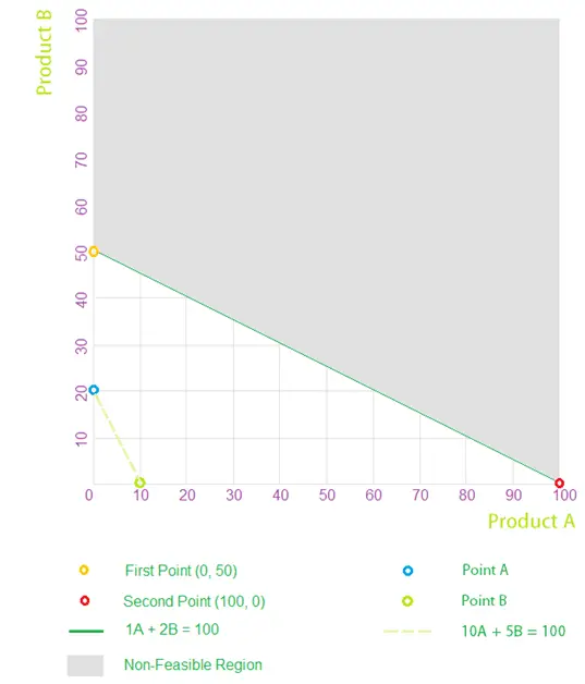
Working
Point A:
10(0) + 5B = 100
B = 100 ÷ 5
B = 20
(0, 20)
Point B:
10(A) + 5(0) = 100
A = 100 ÷ 10
A = 10
(10, 0)
Step 6: Find the optimum point
Optimum point of a linear programming problem always lies on one of the corner points of the graph’s feasible region.
To find the optimum point, you need to slide a ruler across the graph along the gradient of objective function. Where the objective is to maximize (e.g. contribution), you must slide the ruler up to the point within the feasible region which is furthest away from the origin. Conversely, where the objective is to minimize (e.g. cost) you must slide the ruler up to the point within the feasible region that is nearest to the origin. In both cases, you must remember to slide the ruler along the gradient of the objective function line.
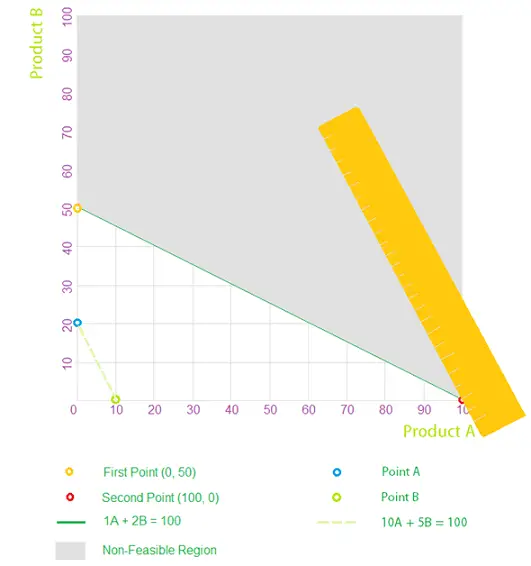
Note that the ruler is parallel to the dotted line (i.e. the objective function line). The red point marked on the graph (100, 0) is the last point that the ruler touches while still remaining in the feasible region and is therefore the optimum point.
Step 7: Find the coordinates of the optimum point
In the above example, the co-ordinates of the optimum point can be identified easily because the point lies on the X-Axis.
If the optimum point of a linear programming problem does not lie on either x or y axis, you can find its co-ordinates by drawing vertical and horizontal lines from the optimum point towards the two axis.